The Three Faces of Bayes

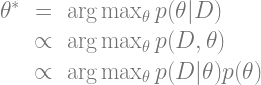
Last summer, I was at a conference having lunch with Hal Daumé III when we got to talking about how “Bayesian” can be a funny and ambiguous term. It seems like the definition should be straightforward: “following the work of English mathematician Rev. Thomas Bayes,” perhaps, or even “uses Bayes’ theorem.” But many methods bearing the reverend’s name or using his theorem aren’t even considered “Bayesian” by his most religious followers. Why is it that Bayesian networks, for example, aren’t considered… y’know… Bayesian?

As I’ve read more outside the fields of machine learning and natural language processing — from psychometrics and environmental biology to hackers who dabble in data science — I’ve noticed three broad uses of the term “Bayesian.” I mentioned to Hal that I wanted to blog about these different uses, and he said it probably would have been more useful about six years ago when being “Bayesian” was all the rage (being “deep” is where it’s at these days). I still think these are useful distinctions, though, so here it is anyway.

I’ll present the three main uses of “Bayesian” as I understand them, all through the lens of a naïve Bayes classifier. I hope you find it useful and interesting!

A Theorem By Any Other Name…

First off, Bayes’ theorem (in some form) is involved in all three takes on “Bayesian.” This 250-year-old staple of statistics gives us a way to estimate the probability of some outcome of interest given some evidence :

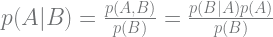
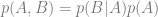
If we care about inferring  from , Bayes’ theorem says this can be done by estimating the joint probability and then dividing by the marginal probability to get the conditional probability . The second equivalence follows from the chain rule: .  is called the prior distribution over , and  is called the posterior distribution over after having observed .

1. Bayesians Against Discrimination

Now briefly consider this photo from the Pittsburgh G20 protests in 2009. That’s me carrying a sign that says “Bayesians Against Discrimination” behind the one and only John Oliver. I don’t think he realized he was in satirical company at the time (photo by Arthur Gretton, more ML protest photos here).

To get the joke, you need to grasp the first interpretation of “Bayesian”: a model that uses Bayes’ theorem to make predictions given some data…

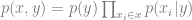
Bayesian networks are probabilistic models that rely on Bayes’ theorem, and a special case is the naïve Bayes classifier. It’s a popular model for text applications like spam filtering. Given a document  as “evidence,” we want to predict the best label  with the highest probability  of given . We can do that using the theorem like so:

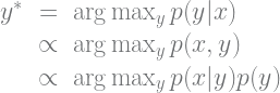
If all we really care about is the best (most probable) , we can ignore the marginal from the denominator of Bayes’ theorem, since it is fixed and constant for all labels (hence the proportional in the second and third lines). The naïvité of naïve Bayes comes from the (not always realistic) assumption that the probability of each word is independent of the others, given . This makes our lives easier by letting us just multiply all the class-conditional word probabilities together in order to estimate the joint probability: . Given a training set of labeled texts (e.g., spam vs. legit email), we can count up all the labels and words to estimate and probabilities into a set of classifier parameters we’ll call . Taken together, the parameters in approximate the joint probability . Then we use Bayes’ theorem to predict class labels for any new document . Nice!

A Bayesian network like naïve Bayes is considered a generative model with a generative story. The generative story for naïve Bayes goes like this:

• to make a document, first sample a class label according to
• then, sample each word in the document according to

This story says we can generate new hypothetical documents because we approximated the full joint distribution . However, for classification we really just care about the conditional distribution , so we need to use Bayes’ theorem. In contrast, discriminative models like logistic regression assume that we don’t care about the joint distribution to begin with, so why not just estimate directly? Bayes’ theorem need not apply.

So the G20 protest joke interprets “Bayesian” to mean generative (not discriminative) modeling. In other words, if we’re Bayesian, we want to model the joint probability of variables and use Bayes’ theorem to make predictions.

(Note: naïve Bayes and logistic regression are considered a “generative-discriminative pair,” since they take the same graphical form, but parameters are estimated differently and have different interpretations; see Ng & Jordan (2002) for more on this.)

2. If You Liked It, Then You Should’ve Put A Prior On It

Now consider this high-profile reaction to our G20 joke:

I confess I don’t understand the “Bayesians against discrimination!” sign. As Ng and Jordan have shown, Bayesians can make good use of both discriminative and generative methods.
~ Peter Norvig (Director of Research at Google)

Sensible as it may seem, the “Bayesian == generative” interpretation is pretty rare, and will probably get you laughed out of the room at a quant-nerd cocktail party (although let’s be honest: these aren’t the best cocktail parties). To understand Norvig’s comment, you need to grasp our second interpretation of “Bayesian”: don’t use Bayes’ theorem for prediction, use it for learning!

Given a training set as “evidence,” the goal of machine learning is to pick the best model with the highest probability . Well, we can do that using Bayes’ theorem, too:

Again, if we just care about the “best” model parameters we can ignore from the denominator of Bayes’ theorem, since the data are fixed and it would be constant anyway. So in this “Bayesian” way of learning, is a function of — the likelihood of the data given the model — and — the “prior” distribution over all possible models. If we think all models are equally likely, we can ignore the prior and just maximize . This is called maximum likelihood estimation (MLE), and that’s essentially how I described naïve Bayes parameter learning in the previous section. Including a prior gives us maximum a posteriori (MAP) estimation: start with a prior distribution and update it to a posterior distribution after seeing some data.

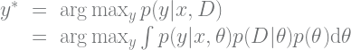
(Note: using Bayes’ theorem for prediction, as we did in the first section, can be considered “MAP inference” because we maximize the posterior . Naïve Bayes parameters include a prior on the class label , but the actual parameter learning was still MLE because we didn’t use a prior on the parameters themselves.)

So why might we prefer MAP over MLE?

1. Maybe the training set is sketchy and we don’t totally trust it. Say we’re building a naïve Bayes spam filter, but for some reason the word “business” shows up in a couple of spams (“Sir or Madam, I need your help in this urgent business transaction….”) but no legit emails. As a result, p(“business”|legit) = zero, and all future messages containing “business” automatically go to the spam folder, no questions asked. This is a kind of overfitting, and it’s pretty lame.
2. Maybe we know something about the problem. Let’s say we have some domain knowledge, like: the phrases “Nigerian prince” and “Viagra” appear more often in spam. We want to incorporate this knowledge, even if it’s not super-strongly represented in our particular training set.
3. Maybe we want the model to be simple and interpretable. Let’s say we care about inspecting and understanding model parameters just as much as we care about making good predictions. If there are a kajillion variables, we might prefer models that ignore most of them, and only keep a handful of meaningful parameters so we can actually examine them before we die.

For these reasons and more, we want to (and are usually able to) formulate a prior for a MAP estimate of . With naïve Bayes, the word probabilities are usually modeled as a multinomial distribution, for which a Dirichlet distribution is the conjugate prior. This means we can add some number of “hallucinated” counts to each parameter for a “smoothed” version of the MLE for MAP estimation. Adding a pseudo-count of one to everything (“Laplace smoothing”) is pretty common, and is a type of uninformative prior called a “symmetric Dirichlet prior.” This is useful for combatting the overfitting spam filter in the first bullet point: p(“business”|legit) will always be positive with this prior, even if it is small. The higher the pseudo-count, the more training data are needed to pry the posterior away from the prior . Adding different pseudo-counts for each parameter yields an “asymmetric Dirichlet prior,” which can be a type of informative prior if we give a boost to words we know about, as with the second bullet (e.g., “Viagra” implies spam).

Back to Norvig’s criticism: under the “Bayesian == MAP estimation” way of thinking, even discriminative models can be Bayesian, if we incorporate priors. We often call this regularization in machine learning, which can help combat overfitting and simplify the model (à la Occam’s razor). For example, L1 regularized regression uses a prior on regression weights that follows a zero-mean Laplace distribution. This encourages sparsity, which aids interpretability in the spirit of the third bullet point above (allowing mere mortals to examine the weights). Similarly, L2 regularization puts a prior on weights that follows a zero-mean Gaussian (Normal) distribution.

(Note: L1 and L2 regularized regression are respectively known as LASSO and ridge regression in statistics circles. So just as different research communities can use the same term — like “Bayesian” — to mean different things, they can also use different terms to mean the same thing! Ever heard of a multinomial logit? No? Well, it’s the same thing as a softmax model, and a polytomous regression, and a maximum-entropy classifier, and a multi-class logistic regression… #FML.)

3. Thou Shalt Not Use Point Estimates

The final, least obvious, and possibly most pedantic use of “Bayesian” stems from the belief that “model parameters should be treated as unobserved random variables about which we have uncertainty, which should therefore be accounted for when making predictions.” Uhmmmm… wha?

OK, to unpack that a bit, notice that up until now we’ve only been concerned with maximizing some posterior probability. In the case of MAP learning in the previous section, our “best guess” parameter estimate is a point estimate: supposedly the best of many possible models. But Bayes’ theorem gives us, in theory, a probability distribution over the entire space of all possible models, and there could be a lot of variance among them! What if our best point estimate spam filter is wrong for a whole group of emails where some other not-the-best point estimate gets it right? Don’t we want to make use of the entire posterior distribution over that Bayes’ theorem can provide?

Some folks do exactly that: integrate out model parameters altogether when making predictions. Odds are, if you meet people who refer to themselves as Bayesian — not just their methods — then this is what they’re talking about. In this way of thinking, the posterior predictive distribution is conditioned only on the input and training data (plus whatever prior you specify):

This is easy enough to do for small, discrete model spaces: just enumerate every possible  in brute-force fashion. For most interesting problems, however, this sort of Bayesian inference is at best computationally gross and at worst mathematically futile. This is why Bayesian networks are considered by some people not to be “Bayesian” at all: for efficiency’s sake, we often just use a point estimate of model parameters to make new inferences.

The good news is that we now have many tricks, such as Markov chain Monte Carlo (MCMC) methods, for sampling from the model posterior to approximate the integral above more efficiently. In particular, Gibbs sampling can be used to make “Bayesian” inferences for a naïve Bayes classifier (in this sense). See Resnik & Hardesty (2010) for a good tutorial.

Conclusion

There you have it! The three faces of Bayes:

1. Generative modeling with Bayes’ theorem for inference,
2. Incorporating a prior for MAP model parameter learning, or
3. Integrating out the model parameters for more “integrated” inference.

So the next time someone starts chatting about “Bayesian” methods at a cocktail party, maybe this post can help you figure out what sense he or she means…

Update (August 30, 2016): It has come to my attention that the image I based my “Three Faces” graphic on above may not even be the face of Bayes! Furthermore, if you think three is bad, by some accounts there are at least 46,656 Varieties of Bayesians. 🙂